Entropy and related measures

Note

The lemon datasets used in this tutorial is composed of EEGLAB files. To use the MNE reader mne.io.read_raw_eeglab(), the pymatreader optional dependency is required. Use the following installation method appropriate for your environment:

• pip install pymatreader

• conda install -c conda-forge pymatreader

Note that an environment created via the MNE installers includes pymatreader by default.

# Authors: Frederic von Wegner <fvwegner@gmail.com>
#          Victor Férat <victor.ferat@live.fr>

import numpy as np
from matplotlib import pyplot as plt
from mne.io import read_raw_eeglab

from pycrostates.cluster import ModKMeans
from pycrostates.datasets import lemon
from pycrostates.segmentation import (
    auto_information_function,
    excess_entropy_rate,
    partial_auto_information_function,
)

Load example data

We load 60 seconds of eyes-closed (EC) resting state data from the Babayan et al.[1] database.

raw_fname = lemon.data_path(subject_id="010021", condition="EC")
raw = read_raw_eeglab(raw_fname, preload=False)
raw.crop(0, 60).load_data()  # crop the dataset to speed up computation
raw.set_eeg_reference("average")  # apply a common average reference

/home/docs/checkouts/readthedocs.org/user_builds/pycrostates/checkouts/latest/tutorials/segmentation/10_entropy.py:47: RuntimeWarning: Limited 1 annotation(s) that were expanding outside the data range.
  raw = read_raw_eeglab(raw_fname, preload=False)
/home/docs/checkouts/readthedocs.org/user_builds/pycrostates/checkouts/latest/tutorials/segmentation/10_entropy.py:47: RuntimeWarning: The data contains 'boundary' events, indicating data discontinuities. Be cautious of filtering and epoching around these events.
  raw = read_raw_eeglab(raw_fname, preload=False)

	General
	Filename(s)	sub-010021_EC.fdt
	MNE object type	RawEEGLAB
	Measurement date	Unknown
	Participant	Unknown
	Experimenter	Unknown
	Acquisition
	Duration	00:01:01 (HH:MM:SS)
	Sampling frequency	250.00 Hz
	Time points	15,001
	Channels
	EEG	61
	Head & sensor digitization	64 points
	Filters
	Highpass	0.00 Hz
	Lowpass	125.00 Hz

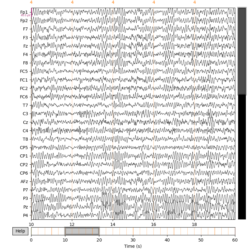
This subject has a posterior dominant rhythm in the alpha frequency band.

raw.plot(duration=10.0, start=10.0, n_channels=25)
plt.show()

Microstate clustering

Perform a clustering into K=5 microstate classes.

ModK = ModKMeans(n_clusters=5, random_state=42)
ModK.fit(raw, n_jobs=2)
ModK.reorder_clusters(order=[4, 2, 0, 3, 1])
ModK.rename_clusters(new_names=["A", "B", "C", "D", "F"])
ModK.plot()
plt.show()

Segmentation

Perform two segmentations, i.e. back-fitting the maps obtained in the previous step, followed by:

• 1. Minimal post-processing (half_window_size=1, min_segment_length=1)

• 2. Temporal smoothing (half_window_size=3, min_segment_length=5)

Once a set of cluster centers has been fitted, it can be used to predict the microstate segmentation with the method pycrostates.cluster.ModKMeans.predict(). It returns either a RawSegmentation or an EpochsSegmentation depending on the object to segment. In this example, the provided instance is a continuous Raw object:

segm_pure = ModK.predict(
    raw,
    reject_by_annotation=True,
    factor=10,
    half_window_size=1,
    min_segment_length=1,
    reject_edges=True,
)

segm_smooth = ModK.predict(
    raw,
    reject_by_annotation=True,
    factor=10,
    half_window_size=5,
    min_segment_length=5,
    reject_edges=True,
)

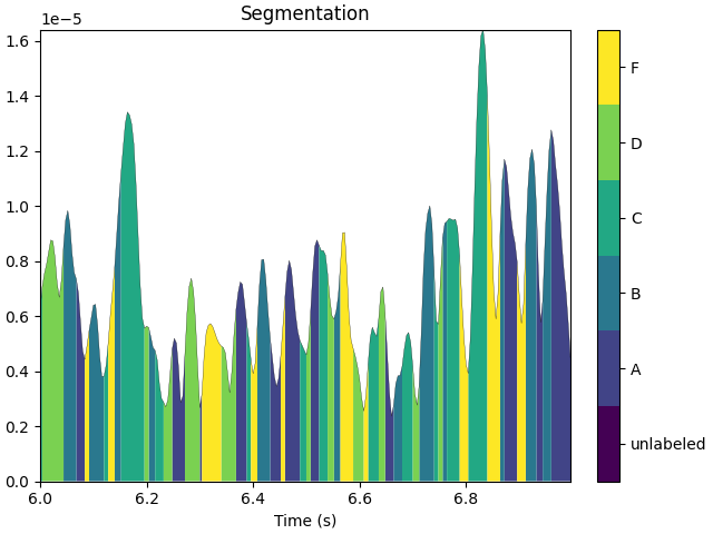
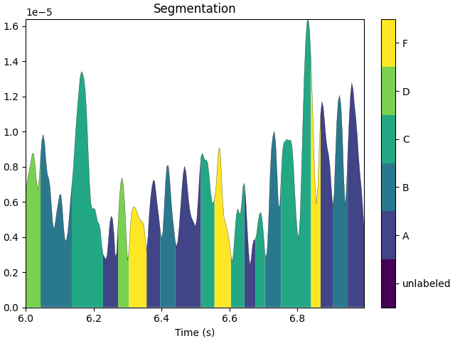
The differences between the non-smoothed (pure) and smoothed microstate sequences can be visualized with the plot method of the segmentation objects.

t0, t1 = 6, 7
segm_pure.plot(tmin=t0, tmax=t1)
segm_smooth.plot(tmin=t0, tmax=t1)
plt.show()

• 
• 

Shannon entropy

The Shannon entropy[2] of the microstate sequence describes how flat the microstate class distribution is. The two extremes are:

• A flat distribution. In this example, the maximum entropy would be observed if each microstate class (A, B, C, D, F) had probability \(p=1/5\). The resulting Shannon entropy would be \(h=log(5)=2.32 bits\).

• A peaked distribution. If any microstate class occurs with probability \(p=1\), and all other classes with probability \(p=0\), the resulting Shannon entropy would achieve its minimum value of \(h=0\) bits.

In this example, we observe that smoothing leads to a slight entropy reduction.

h_pure = segm_pure.entropy(ignore_repetitions=False)
h_smooth = segm_smooth.entropy(ignore_repetitions=False)
print(f"Microstate sequence without smoothing, Shannon entropy h = {h_pure:.2f} bits")
print(f"Microstate sequence with    smoothing, Shannon entropy h = {h_smooth:.2f} bits")

Microstate sequence without smoothing, Shannon entropy h = 2.30 bits
Microstate sequence with    smoothing, Shannon entropy h = 2.26 bits

Entropy rate and excess entropy

The entropy rate of the microstate sequence is a measure of its Kolmogorov complexity while excess entropy measures statistical complexity. High entropy rate (or high Kolmogorov complexity) means that the next microstate label is less predictable, based on the sequence history.

History length is provided as a free parameter history_length when calling the excess_entropy_rate and is given in number of samples. The excess_entropy_rate function performs a linear fit to joint entropy values across different history lengths and returns two parameters; the slope parameter corresponds to the entropy rate, the y-axis intersection to excess entropy.

This procedure is illustrated below. Further details are given in von Wegner et al.[3].

h_length = 9  # history_length
a, b, residuals, lags, joint_entropies = excess_entropy_rate(
    segm_pure, history_length=h_length, ignore_repetitions=False
)
print(f"Entropy rate: {a:.3f} bits/sample.")
print(f"Excess entropy: {b:.3f} bits.")

# joint entropy plot from which excess entropy and entropy rate are calculated
plt.figure()
plt.plot(lags, joint_entropies, "-sk")
plt.plot(lags, a * lags + b, "-b")
plt.xlabel("lag (samples)")
plt.ylabel("joint entropy (bit)")
plt.title("Entropy rate & excess entropy")
plt.show()

Entropy rate: 1.036 bits/sample.
Excess entropy: 1.428 bits.

We can now test how microstate sequence (Kolmogorov) complexity changes with pre-processing:

• no smoothing, full microstate sequence (duplicates not removed)

• smoothing, full microstate sequence (duplicates not removed)

• no smoothing, microstate jump sequence (duplicates removed)

• smoothing, microstate jump sequence (duplicates removed)

Smoothing makes microstate sequences more predictable (less complex), removing duplicates makes sequences less predictable (more complex).

We can ignore state repetitions (i.e. self-transitions) by setting the argument ignore_repetitions to True. This is useful when you don’t want to take state duration into account.

er_pure, _, _, _, _ = excess_entropy_rate(
    segm_pure, history_length=h_length, ignore_repetitions=False
)
er_smooth, _, _, _, _ = excess_entropy_rate(
    segm_smooth, history_length=h_length, ignore_repetitions=False
)
er_pure_jump, _, _, _, _ = excess_entropy_rate(
    segm_pure, history_length=h_length, ignore_repetitions=True
)
er_smooth_jump, _, _, _, _ = excess_entropy_rate(
    segm_smooth, history_length=h_length, ignore_repetitions=True
)
print(
    f"1. Microstate      sequence without smoothing, entropy rate: {er_pure:.2f} bits/sample"
)
print(
    f"2. Microstate      sequence with    smoothing, entropy rate: {er_smooth:.2f} bits/sample"
)
print(
    f"3. Microstate jump sequence without smoothing, entropy rate: {er_pure_jump:.2f} bits/sample"
)
print(
    f"4. Microstate jump sequence with    smoothing, entropy rate: {er_smooth_jump:.2f} bits/sample"
)

1. Microstate      sequence without smoothing, entropy rate: 1.04 bits/sample
2. Microstate      sequence with    smoothing, entropy rate: 0.43 bits/sample
3. Microstate jump sequence without smoothing, entropy rate: 1.20 bits/sample
4. Microstate jump sequence with    smoothing, entropy rate: 0.93 bits/sample

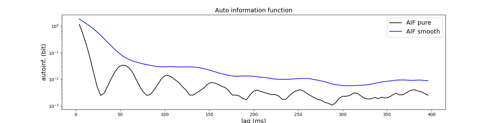
Autoinformation function

The autoinformation function (AIF) is the information-theoretic analogy to the autocorrelation function (ACF) for numerical timeseries. The autoinformation coefficient at time lag \(k\) is the information shared between microstate labels \(k\) time samples apart. Mathematically, it is computed as the mutual information between the microstate label \(X_t\) at time \(t\), and the label \(X_{t+k}\) at \(t+k\), averaged across the whole sequence: \(H(X_{t+k}) - H(X_{t+k} \vert X_{t})\).

Below, we compare the AIF of microstate sequences with and without smoothing. Smoothing increases overall temporal dependencies and removes microstate oscillations (AIF peaks at 50, 100, 150 ms) that are visible in the minimally pre-processed sequence.

We compute the AIF for the full microstate sequence with and without smoothing

lags1 = np.arange(1, 100)
lags, ai_pure = auto_information_function(
    segm_pure, lags=lags1, ignore_repetitions=False, n_jobs=2
)
lags, ai_smooth = auto_information_function(
    segm_smooth, lags=lags1, ignore_repetitions=False, n_jobs=2
)

lags_ms = lags * 1000 / raw.info["sfreq"]  # convert samples in milliseconds
plt.figure(figsize=(16, 4))
plt.semilogy(lags_ms, ai_pure, "-k", label="AIF pure")
plt.semilogy(lags_ms, ai_smooth, "-b", label="AIF smooth")
plt.legend(loc="upper right", fontsize=14)
plt.xlabel("lag (ms)", fontsize=14)
plt.ylabel("autoinf. (bit)", fontsize=14)
plt.title("Auto information function", fontsize=14)
plt.show()

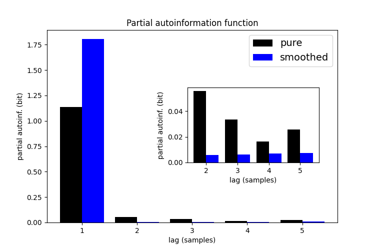
Partial autoinformation

Partial autoinformation (PAI) describes the dependence between microstate sequence labels \(k\) samples apart, removing the influence of all intermediate labels. The autoinformation function does not account for the effect of intermediate time steps. PAI is computationally more expensive and it is recommended to start with a low number of lags (e.g. 5). PAI coefficients can identify (first-order) Markov processes as their PAI coefficients are zero for lags \(k \ge 2\).

Below, we compare the PAI coefficients of microstate sequences with and without smoothing. Smoothing shifts temporal dependencies towards the first time lag, i.e. smoothing makes sequences more Markovian.

lags_paif = np.arange(1, 6)
lags2, pai_pure = partial_auto_information_function(
    segm_pure, lags=lags_paif, ignore_repetitions=False, n_jobs=1
)
lags2, pai_smooth = partial_auto_information_function(
    segm_smooth, lags=lags_paif, ignore_repetitions=False, n_jobs=1
)

w = 0.4
wh = w / 2

fig = plt.figure(figsize=(7.5, 5))
ax = plt.gca()
ax.bar(lags_paif - wh, pai_pure, width=w, color="k", label="pure")
ax.bar(lags_paif + wh, pai_smooth, width=w, color="b", label="smoothed")
ax.legend(loc="upper right", fontsize=14)
ax.set_xlabel("lag (samples)")
ax.set_ylabel("partial autoinf. (bit)")

offset = 1
left, bottom, width, height = [0.5, 0.35, 0.35, 0.3]
axin = fig.add_axes([left, bottom, width, height])
axin.bar(lags_paif[offset:] - wh, pai_pure[offset:], color="k", width=w)
axin.bar(lags_paif[offset:] + wh, pai_smooth[offset:], color="b", width=w)
axin.set_xlabel("lag (samples)")
axin.set_ylabel("partial autoinf. (bit)")

ax.set_title("Partial autoinformation function")
plt.show()

References

[1]

Anahit Babayan, Miray Erbey, and Deniz Kumral. A mind-brain-body dataset of MRI, EEG, cognition, emotion, and peripheral physiology in young and old adults. Scientific Data, 6(1):180308, 2019. doi:10.1038/sdata.2018.308.

[2]

Claude E Shannon. A mathematical theory of communication. The Bell system technical journal, 27(3):379–423, 1948. doi:10.1002/j.1538-7305.1948.tb01338.x.

[3]

Frederic von Wegner, Milena Wiemers, Gesine Hermann, Inken Tödt, Enzo Tagliazucchi, and Helmut Laufs. Complexity measures for eeg microstate sequences: concepts and algorithms. Brain Topography, 2023. doi:10.1007/s10548-023-01006-2.

Estimated memory usage: 270 MB