Note

Go to the end to download the full example code.

Microstate Segmentation#

This tutorial introduces the concept of segmentation.

Segmentation#

We start by fitting a modified K-means (ModKMeans) with a sample dataset. For more details about fitting a clustering algorithm, please refer to this tutorial.

Note

The lemon datasets used in this tutorial is composed of EEGLAB files. To use the MNE reader mne.io.read_raw_eeglab(), the pymatreader optional dependency is required. Use the following installation method appropriate for your environment:

pip install pymatreader
conda install -c conda-forge pymatreader

Note that an environment created via the MNE installers includes pymatreader by default.

Note

This tutorial uses seaborn for enhanced visualization. Use the following installation method appropriate for your environment:

pip install seaborn
conda install -c conda-forge seaborn

import numpy as np
import seaborn as sns
from matplotlib import pyplot as plt
from mne.io import read_raw_eeglab

from pycrostates.cluster import ModKMeans
from pycrostates.datasets import lemon

raw_fname = lemon.data_path(subject_id="010017", condition="EC")
raw = read_raw_eeglab(raw_fname, preload=False)
raw.crop(0, 60)  # crop the dataset to speed up computation
raw.load_data()
raw.set_eeg_reference("average")  # Apply a common average reference

ModK = ModKMeans(n_clusters=5, random_state=42)
ModK.fit(raw, n_jobs=2)
ModK.reorder_clusters(order=[4, 1, 3, 2, 0])
ModK.rename_clusters(new_names=["A", "B", "C", "D", "F"])
ModK.plot()

/home/docs/checkouts/readthedocs.org/user_builds/pycrostates/checkouts/latest/tutorials/segmentation/00_segmentation.py:52: RuntimeWarning: Limited 1 annotation(s) that were expanding outside the data range.
  raw = read_raw_eeglab(raw_fname, preload=False)
/home/docs/checkouts/readthedocs.org/user_builds/pycrostates/checkouts/latest/tutorials/segmentation/00_segmentation.py:52: RuntimeWarning: The data contains 'boundary' events, indicating data discontinuities. Be cautious of filtering and epoching around these events.
  raw = read_raw_eeglab(raw_fname, preload=False)

<Figure size 1500x300 with 5 Axes>

Once a set of cluster centers has been fitted, It can be used to predict the microstate segmentation with the method pycrostates.cluster.ModKMeans.predict(). It returns either a RawSegmentation or an EpochsSegmentation depending on the object to segment. Below, the provided instance is a continuous Raw object:

segmentation = ModK.predict(
    raw,
    reject_by_annotation=True,
    factor=10,
    half_window_size=10,
    min_segment_length=5,
    reject_edges=True,
)

The factor and half_window_size arguments control the smoothing algorithm introduced by Pascual Marqui[1]. This algorithm corrects wrong label assignments which occur during periods of low signal to noise ratio. For each timepoint, it takes into account the label of the neighboring segments to favor an assignment that increases label continuity (i.e. long segments). The factor parameter controls the strength of the influence of the neighboring segments while the half_window_size parameter controls how far (in time) neighboring segments have an influence.

A second outlier rejection algorithm can be used on top. Controlled by the min_segment_length parameter, it re-assigns segments of short duration to their neighboring segments.

The label of each datapoints are stored in the labels attribute.

segmentation.labels

array([-1, -1, -1, ..., -1, -1, -1], shape=(15001,))

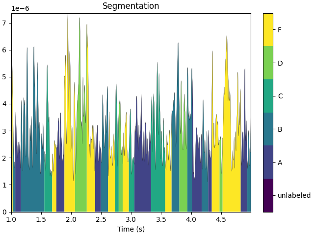
The segmentation can be visualized with the method plot().

segmentation.plot(tmin=1, tmax=5)
plt.show()

Microstates parameters#

The usual parameters used in microstate analysis can be computed with the method compute_parameters(). This method returns a dict with a key corresponding to each combination of cluster_center name and parameter name.

parameters = segmentation.compute_parameters()
parameters

{'A_mean_corr': np.float64(0.5346414252737214), 'A_gev': np.float64(0.049431508577113134), 'A_occurrences': 1.4867031939061874, 'A_timecov': np.float64(0.14947213684351196), 'A_meandurs': np.float64(0.10053932584269663), 'B_mean_corr': np.float64(0.6244742905388542), 'B_gev': np.float64(0.10880756109587916), 'B_occurrences': 1.7873847387411466, 'B_timecov': np.float64(0.20680208472537753), 'B_meandurs': np.float64(0.11570093457943927), 'C_mean_corr': np.float64(0.6855601832541897), 'C_gev': np.float64(0.2282498250281446), 'C_occurrences': 1.73727114793532, 'C_timecov': np.float64(0.245088868101029), 'C_meandurs': np.float64(0.14107692307692307), 'D_mean_corr': np.float64(0.5374672855194499), 'D_gev': np.float64(0.05464069684808019), 'D_occurrences': 1.620339436055058, 'D_timecov': np.float64(0.17098757182948016), 'D_meandurs': np.float64(0.10552577319587629), 'F_mean_corr': np.float64(0.625669782839815), 'F_gev': np.float64(0.1301698676266293), 'F_occurrences': 1.9544300414272349, 'F_timecov': np.float64(0.22764933850060137), 'F_meandurs': np.float64(0.11647863247863248), 'unlabeled': 0.0023331777881474567}

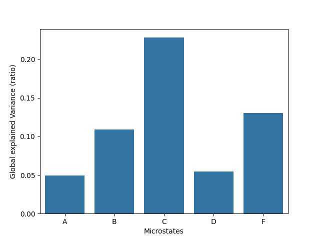
Global Explained Variance#

gev is the total explained variance expressed by a given state. It is computed as the sum of global explained variance values of each time point assigned to a given state.

x = ModK.cluster_names
y = [parameters[elt + "_gev"] for elt in x]

ax = sns.barplot(x=x, y=y)
ax.set_xlabel("Microstates")
ax.set_ylabel("Global explained Variance (ratio)")
plt.show()

Mean correlation#

mean_corr corresponds to the mean correlation value of each time point assigned to a given state.

x = ModK.cluster_names
y = [parameters[elt + "_mean_corr"] for elt in x]

ax = sns.barplot(x=x, y=y)
ax.set_xlabel("Microstates")
ax.set_ylabel("Mean correlation")
plt.show()

Time coverage#

timecov corresponds to the proportion of time during which a given state is active.

x = ModK.cluster_names
y = [parameters[elt + "_timecov"] for elt in x]

ax = sns.barplot(x=x, y=y)
ax.set_xlabel("Microstates")
ax.set_ylabel("Time Coverage (ratio)")
plt.show()

Mean durations#

meandurs corresponds to the mean temporal duration of segments assigned to a given state.

x = ModK.cluster_names
y = [parameters[elt + "_meandurs"] for elt in x]

ax = sns.barplot(x=x, y=y)
ax.set_xlabel("Microstates")
ax.set_ylabel("Mean duration (s)")
plt.show()

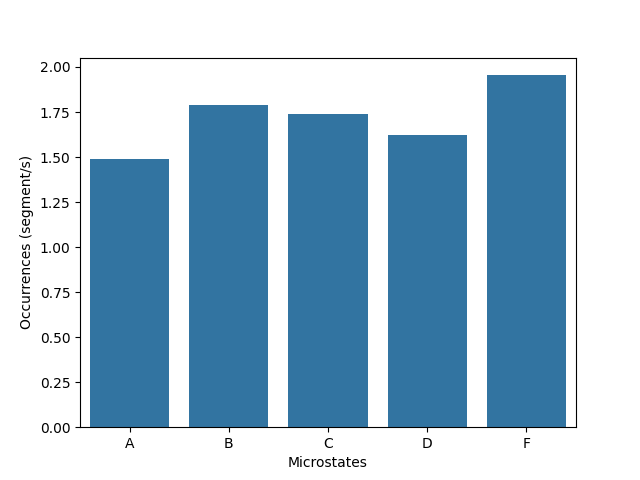
Occurrence per second#

occurrences indicates the mean number of segments assigned to a given state per second. This metrics is expressed in segment per second.

x = ModK.cluster_names
y = [parameters[elt + "_occurrences"] for elt in x]

ax = sns.barplot(x=x, y=y)
ax.set_xlabel("Microstates")
ax.set_ylabel("Occurrences (segment/s)")
plt.show()

Distributions#

By setting return_dist=True the underlying distributions used to computed those metrics are returned.

parameters = segmentation.compute_parameters(return_dist=True)
parameters

{'A_mean_corr': np.float64(0.5346414252737214), 'A_gev': np.float64(0.049431508577113134), 'A_occurrences': 1.4867031939061874, 'A_timecov': np.float64(0.14947213684351196), 'A_meandurs': np.float64(0.10053932584269663), 'A_dist_corr': array([ 0.46121789,  0.52395882,  0.54376569, ..., -0.77822393,
       -0.7863559 , -0.7572945 ], shape=(2237,)), 'A_dist_gev': array([4.78813181e-06, 1.18442487e-05, 1.63422005e-05, ...,
       1.15233123e-05, 9.85485151e-06, 1.23715453e-05], shape=(2237,)), 'A_dist_durs': array([0.096, 0.136, 0.096, 0.28 , 0.164, 0.06 , 0.112, 0.044, 0.148,
       0.076, 0.064, 0.08 , 0.104, 0.092, 0.052, 0.096, 0.056, 0.084,
       0.068, 0.048, 0.052, 0.108, 0.072, 0.044, 0.06 , 0.128, 0.1  ,
       0.14 , 0.064, 0.076, 0.056, 0.116, 0.212, 0.18 , 0.06 , 0.08 ,
       0.052, 0.104, 0.06 , 0.064, 0.16 , 0.052, 0.08 , 0.104, 0.084,
       0.044, 0.168, 0.176, 0.056, 0.052, 0.084, 0.068, 0.052, 0.232,
       0.096, 0.056, 0.064, 0.104, 0.168, 0.096, 0.088, 0.056, 0.056,
       0.056, 0.104, 0.072, 0.076, 0.052, 0.08 , 0.164, 0.312, 0.148,
       0.104, 0.06 , 0.068, 0.08 , 0.136, 0.076, 0.276, 0.216, 0.068,
       0.08 , 0.06 , 0.108, 0.12 , 0.064, 0.112, 0.204, 0.072]), 'B_mean_corr': np.float64(0.6244742905388542), 'B_gev': np.float64(0.10880756109587916), 'B_occurrences': 1.7873847387411466, 'B_timecov': np.float64(0.20680208472537753), 'B_meandurs': np.float64(0.11570093457943927), 'B_dist_corr': array([0.39588089, 0.48685777, 0.53990163, ..., 0.29996699, 0.30217753,
       0.37320483], shape=(3095,)), 'B_dist_gev': array([5.39912177e-06, 8.85977991e-06, 1.06100313e-05, ...,
       4.14797890e-06, 6.61139792e-06, 1.20001971e-05], shape=(3095,)), 'B_dist_durs': array([0.144, 0.236, 0.044, 0.388, 0.12 , 0.132, 0.076, 0.108, 0.136,
       0.176, 0.4  , 0.06 , 0.36 , 0.184, 0.108, 0.048, 0.16 , 0.064,
       0.096, 0.092, 0.076, 0.104, 0.08 , 0.104, 0.064, 0.08 , 0.308,
       0.088, 0.092, 0.076, 0.156, 0.072, 0.116, 0.16 , 0.072, 0.1  ,
       0.088, 0.156, 0.116, 0.076, 0.056, 0.064, 0.06 , 0.116, 0.072,
       0.144, 0.12 , 0.076, 0.084, 0.072, 0.088, 0.112, 0.084, 0.172,
       0.064, 0.256, 0.132, 0.16 , 0.128, 0.132, 0.212, 0.096, 0.072,
       0.124, 0.088, 0.064, 0.064, 0.072, 0.236, 0.176, 0.056, 0.112,
       0.112, 0.052, 0.06 , 0.072, 0.208, 0.064, 0.18 , 0.164, 0.148,
       0.136, 0.068, 0.104, 0.1  , 0.04 , 0.072, 0.112, 0.064, 0.192,
       0.064, 0.076, 0.048, 0.08 , 0.292, 0.1  , 0.068, 0.1  , 0.044,
       0.072, 0.096, 0.124, 0.072, 0.052, 0.092, 0.104, 0.068]), 'C_mean_corr': np.float64(0.6855601832541897), 'C_gev': np.float64(0.2282498250281446), 'C_occurrences': 1.73727114793532, 'C_timecov': np.float64(0.245088868101029), 'C_meandurs': np.float64(0.14107692307692307), 'C_dist_corr': array([-0.75398016, -0.79462083, -0.77615933, ...,  0.91183077,
        0.88752534,  0.85336098], shape=(3668,)), 'C_dist_gev': array([9.62107886e-06, 1.07964953e-05, 7.73967640e-06, ...,
       1.22361899e-04, 1.34220541e-04, 1.31921192e-04], shape=(3668,)), 'C_dist_durs': array([0.156, 0.088, 0.132, 0.064, 0.092, 0.236, 0.112, 0.348, 0.12 ,
       0.2  , 0.096, 0.06 , 0.092, 0.084, 0.192, 0.08 , 0.244, 0.16 ,
       0.076, 0.384, 0.124, 0.096, 0.104, 0.12 , 0.172, 0.16 , 0.084,
       0.048, 0.052, 0.144, 0.068, 0.128, 0.044, 0.168, 0.128, 0.064,
       0.196, 0.068, 0.16 , 0.14 , 0.052, 0.084, 0.104, 0.164, 0.076,
       0.212, 0.064, 0.104, 0.096, 0.132, 0.12 , 0.108, 0.088, 0.056,
       0.348, 0.06 , 0.236, 0.064, 0.124, 0.16 , 0.052, 0.072, 0.056,
       0.808, 0.092, 0.072, 0.052, 0.132, 0.048, 0.072, 0.192, 0.052,
       0.112, 0.12 , 0.428, 0.152, 0.092, 0.076, 0.316, 0.156, 0.156,
       0.06 , 0.124, 0.176, 0.112, 0.196, 0.056, 0.724, 0.156, 0.196,
       0.044, 0.1  , 0.104, 0.364, 0.232, 0.044, 0.1  , 0.104, 0.128,
       0.204, 0.044, 0.048, 0.184, 0.128]), 'D_mean_corr': np.float64(0.5374672855194499), 'D_gev': np.float64(0.05464069684808019), 'D_occurrences': 1.620339436055058, 'D_timecov': np.float64(0.17098757182948016), 'D_meandurs': np.float64(0.10552577319587629), 'D_dist_corr': array([-0.54319309, -0.70981071, -0.73585997, ...,  0.67774271,
        0.60101256,  0.47999274], shape=(2559,)), 'D_dist_gev': array([3.20283960e-06, 8.82749548e-06, 1.65314024e-05, ...,
       1.46932839e-05, 7.62252649e-06, 3.72550043e-06], shape=(2559,)), 'D_dist_durs': array([0.108, 0.196, 0.068, 0.132, 0.052, 0.056, 0.056, 0.096, 0.076,
       0.08 , 0.12 , 0.136, 0.068, 0.128, 0.488, 0.088, 0.044, 0.08 ,
       0.06 , 0.06 , 0.112, 0.08 , 0.192, 0.188, 0.128, 0.048, 0.1  ,
       0.188, 0.108, 0.096, 0.112, 0.044, 0.104, 0.08 , 0.072, 0.064,
       0.072, 0.12 , 0.072, 0.092, 0.112, 0.152, 0.072, 0.18 , 0.128,
       0.108, 0.044, 0.112, 0.064, 0.16 , 0.084, 0.104, 0.132, 0.084,
       0.068, 0.168, 0.12 , 0.076, 0.124, 0.12 , 0.088, 0.052, 0.112,
       0.052, 0.056, 0.044, 0.192, 0.112, 0.084, 0.136, 0.08 , 0.104,
       0.064, 0.128, 0.2  , 0.052, 0.112, 0.068, 0.048, 0.056, 0.052,
       0.092, 0.08 , 0.06 , 0.056, 0.108, 0.096, 0.436, 0.084, 0.108,
       0.152, 0.08 , 0.06 , 0.076, 0.072, 0.192, 0.116]), 'F_mean_corr': np.float64(0.625669782839815), 'F_gev': np.float64(0.1301698676266293), 'F_occurrences': 1.9544300414272349, 'F_timecov': np.float64(0.22764933850060137), 'F_meandurs': np.float64(0.11647863247863248), 'F_dist_corr': array([0.78013258, 0.49291192, 0.37530039, ..., 0.62120228, 0.59793133,
       0.54647673], shape=(3407,)), 'F_dist_gev': array([1.01064927e-05, 3.95582659e-06, 2.93982673e-06, ...,
       3.70567777e-05, 3.25952585e-05, 2.52818999e-05], shape=(3407,)), 'F_dist_durs': array([0.072, 0.144, 0.068, 0.176, 0.14 , 0.112, 0.1  , 0.104, 0.128,
       0.3  , 0.064, 0.08 , 0.064, 0.048, 0.216, 0.148, 0.084, 0.116,
       0.084, 0.104, 0.064, 0.08 , 0.044, 0.084, 0.096, 0.044, 0.044,
       0.072, 0.076, 0.108, 0.116, 0.116, 0.16 , 0.072, 0.112, 0.12 ,
       0.092, 0.048, 0.068, 0.084, 0.088, 0.508, 0.056, 0.076, 0.104,
       0.316, 0.12 , 0.088, 0.364, 0.124, 0.06 , 0.196, 0.108, 0.092,
       0.06 , 0.1  , 0.168, 0.196, 0.096, 0.08 , 0.068, 0.1  , 0.08 ,
       0.16 , 0.1  , 0.048, 0.128, 0.14 , 0.088, 0.072, 0.06 , 0.196,
       0.088, 0.16 , 0.284, 0.288, 0.08 , 0.12 , 0.136, 0.08 , 0.072,
       0.092, 0.096, 0.22 , 0.104, 0.064, 0.068, 0.08 , 0.056, 0.104,
       0.084, 0.104, 0.124, 0.08 , 0.092, 0.08 , 0.04 , 0.268, 0.084,
       0.324, 0.1  , 0.072, 0.064, 0.068, 0.104, 0.168, 0.06 , 0.132,
       0.088, 0.08 , 0.112, 0.172, 0.156, 0.072, 0.072, 0.276, 0.068]), 'unlabeled': 0.0023331777881474567}

For example, the distribution of C segment durations can be plotted.

sns.displot(parameters["C_dist_durs"], stat="probability", bins=30)
plt.show()

Or it can be used to compute other custom metrics from the segmentation. For instance, the median.

median = np.median(parameters["C_dist_durs"])
print(f"Microstate C segments have a median duration of {median:.2f}s.")

Microstate C segments have a median duration of 0.11s.

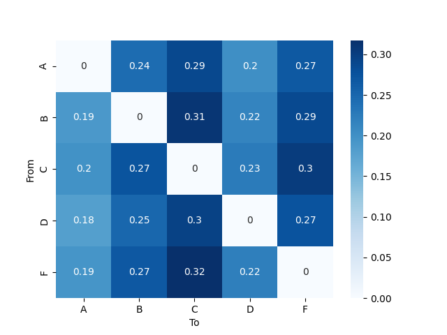
Transition probabilities#

The obsered transition probabilities (T) can be retrieved with the method compute_transition_matrix().

T_observed = segmentation.compute_transition_matrix()

This method returns a array of shape (n_clusters, n_clusters) containing the value corresponding to the chosen statistic:

count will return the number of transitions observed.
probability and proportion will both return the normalized transition probability.
percent will return the normalized transition probability as a percentage.

The rows of T correspond to the "from" state while the columns correspond to the "to" state.

Note

array are 0-indexed, thus T[1, 2] encodes the transition from the second to the third state (B to C in this tutorial).

Note

The transition from and to unlabeled segments are ignored and not taken into account during normalization.

ax = sns.heatmap(
    T_observed,
    annot=True,
    cmap="Blues",
    xticklabels=segmentation.cluster_names,
    yticklabels=segmentation.cluster_names,
)
ax.set_ylabel("From")
ax.set_xlabel("To")
plt.show()

It is however important to take into account the time coverage of each microstate in order to interpret this matrix. The more a state is present, the more there is a chance that a transition towards this state is observed without reflecting any particular dynamics in state transitions.

pycrostates has the possibility to generate a theoretical transition matrix for a given segmentation with the method compute_expected_transition_matrix(). This transition matrix is based on segments counts of each state present in the segmentation but ignores the temporal dynamics (effectively randomizing the transition order).

T_expected = segmentation.compute_expected_transition_matrix()
ax = sns.heatmap(
    T_expected,
    annot=True,
    cmap="Blues",
    xticklabels=segmentation.cluster_names,
    yticklabels=segmentation.cluster_names,
)
ax.set_ylabel("From")
ax.set_xlabel("To")
plt.show()

The difference between the observed transition probability matrix T_observed and the theoretical transition probability matrix T_expected reveals particular dynamic present in the segmentation. Here we observe that the transition from state B to state A appears in larger proportion than expected while the transition from state B to state C is less observed than expected.

ax = sns.heatmap(
    T_observed - T_expected,
    annot=True,
    cmap="RdBu_r",
    vmin=-0.15,
    vmax=0.15,
    xticklabels=segmentation.cluster_names,
    yticklabels=segmentation.cluster_names,
)
ax.set_ylabel("From")
ax.set_xlabel("To")
plt.show()

References#

Total running time of the script: (0 minutes 26.665 seconds)

Estimated memory usage: 231 MB

Gallery generated by Sphinx-Gallery