
Note
Go to the end to download the full example code.
The ModKMeans object#
This tutorial introduces the main clustering object
pycrostates.cluster.ModKMeans structure in detail. The Modified
K-means algorithm is based on Pascual-Marqui et al.[1].
Note
The lemon datasets used in this tutorial is composed of EEGLAB files. To
use the MNE reader mne.io.read_raw_eeglab(), the pymatreader
optional dependency is required. Use the following installation method
appropriate for your environment:
pip install pymatreaderconda install -c conda-forge pymatreader
Note that an environment created via the MNE installers includes
pymatreader by default.
from mne.io import read_raw_eeglab

from pycrostates.cluster import ModKMeans
from pycrostates.datasets import lemon


# load sample dataset
raw_fname = lemon.data_path(subject_id="010017", condition="EC")
raw = read_raw_eeglab(raw_fname, preload=True)
raw.crop(0, 10)  # crop the dataset to speed up computation
raw.pick("eeg")  # select EEG channels
raw.set_eeg_reference("average")  # Apply a common average reference
/home/docs/checkouts/readthedocs.org/user_builds/pycrostates/checkouts/latest/tutorials/cluster/00_modK.py:35: RuntimeWarning: Limited 1 annotation(s) that were expanding outside the data range.
  raw = read_raw_eeglab(raw_fname, preload=True)
/home/docs/checkouts/readthedocs.org/user_builds/pycrostates/checkouts/latest/tutorials/cluster/00_modK.py:35: RuntimeWarning: The data contains 'boundary' events, indicating data discontinuities. Be cautious of filtering and epoching around these events.
  raw = read_raw_eeglab(raw_fname, preload=True)
The modified K-means[1] can be instantiated with the
number of cluster centers n_clusters to fit. By default, the
modified K-means will only work with EEG data, but other channel types can be
selected with the picks argument.
Note
A K-means algorithm starts with a random initialization. Thus, 2 separate
fit will not yield the same cluster centers. To achieve
reproductible fits, the random_state argument can be used.
n_clusters = 5
ModK = ModKMeans(n_clusters=n_clusters, random_state=42)
After creating a ModKMeans, the next step is to
fit the model. In other words, fitting a clustering algorithm will determine
the microstate maps, also called cluster centers. A clustering
algorithm can be fitted with Raw,
Epochs or ChData objects.
Note
Fitting a clustering algorithm is a computationally expensive operation.
Depending on your configuration, you can change the argument n_jobs
to take advantage of multiprocessing to reduce computation time.
ModK.fit(raw, n_jobs=5)
Now that our algorithm is fitted, we can visualize the
cluster centers, also called microstate maps or microstate
topographies using pycrostates.cluster.ModKMeans.plot().
Setting show_gradient will plot a line between maximum and minimum
value of each :topography to help visualization.
ModK.plot(show_gradient=True)
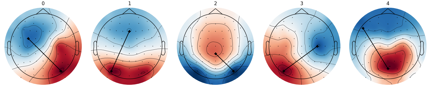
<Figure size 1500x300 with 5 Axes>
The cluster centers can be retrieved as a numpy array with the
cluster_centers_ attribute.
array([[-0.10613817, -0.08201757, -0.12199506, -0.18139598, -0.15155429,
        -0.0663304 ,  0.02897557, -0.14330831, -0.18287982, -0.04394161,
         0.08147253, -0.09112043, -0.17166961, -0.08167475,  0.18571105,
         0.14984234, -0.08960343, -0.05970102,  0.07963704,  0.20116081,
        -0.13068572, -0.01966152, -0.02754429,  0.04342553,  0.17641103,
         0.21959322,  0.05706008,  0.07466215,  0.11798016,  0.19335687,
         0.18025677, -0.1144574 , -0.1478337 , -0.09806771, -0.04387633,
        -0.17137089, -0.18059281, -0.11470747, -0.02275574, -0.12266696,
        -0.19038825,  0.06154834,  0.09349215, -0.12954759, -0.13551292,
         0.03178528,  0.17005063, -0.06435352, -0.10106101, -0.00582698,
         0.17539028,  0.17856175, -0.0303554 ,  0.00050519,  0.10891339,
         0.21417162,  0.03736816,  0.04401132,  0.09312374,  0.18100948,
         0.24512021],
       [-0.13111746, -0.12902983, -0.11675051, -0.15042743, -0.16057124,
        -0.1403919 , -0.09526587, -0.08700381, -0.12771863, -0.1217802 ,
        -0.08104217, -0.0239761 , -0.05611484, -0.09596225, -0.03857956,
        -0.01434362,  0.03886455, -0.0018377 , -0.00541398,  0.04019904,
        -0.15093261,  0.14666805,  0.11686381,  0.07052023,  0.10434424,
         0.13091987,  0.16818435,  0.23991   ,  0.2183577 ,  0.23749697,
         0.16065367, -0.12242205, -0.146566  , -0.14186211, -0.11287111,
        -0.13646411, -0.15545744, -0.15299391, -0.12082361, -0.07459982,
        -0.11163429, -0.09491519, -0.05882318, -0.03486554, -0.07277418,
        -0.06587263, -0.02630238,  0.05202749,  0.01674379, -0.0182837 ,
         0.02217596,  0.05108456,  0.15117688,  0.08485902,  0.07661277,
         0.13336997,  0.27111671,  0.22909926,  0.17786281,  0.205983  ,
         0.23069625],
       [ 0.02779826,  0.03672887, -0.01403513,  0.08561708,  0.12284625,
         0.09263314, -0.01734032,  0.02030784,  0.14198503,  0.1391721 ,
         0.01744079, -0.08370413,  0.10970859,  0.17051393,  0.09571316,
        -0.07978598, -0.02033802,  0.15985952,  0.14735075, -0.01071003,
         0.08177897, -0.20210553,  0.00769019,  0.13026738,  0.01006383,
        -0.20961216, -0.29306345, -0.21966413, -0.16913333, -0.20494208,
        -0.27757552,  0.00050768,  0.06783559,  0.07105905,  0.02605742,
         0.04486   ,  0.11633317,  0.12026605,  0.04057292, -0.02651827,
         0.09721272,  0.09415869, -0.04232562,  0.00503379,  0.1622934 ,
         0.15225462,  0.00137598, -0.13584456,  0.08847654,  0.17401177,
         0.07749566, -0.14216958, -0.11198173,  0.0924721 ,  0.09103009,
        -0.12064577, -0.28421354, -0.0990506 ,  0.01412113, -0.07116736,
        -0.29897722],
       [-0.04938093, -0.07785227,  0.00770551,  0.01101049, -0.05837494,
        -0.12745891, -0.15698158,  0.06574787,  0.03392793, -0.12405229,
        -0.18658613,  0.11186122,  0.12852662, -0.04732016, -0.23913259,
        -0.1712453 ,  0.15846057,  0.04256348, -0.10098047, -0.1684352 ,
        -0.05965646,  0.22080474,  0.16657397,  0.02944206, -0.07509873,
        -0.06890225,  0.21737555,  0.2243419 ,  0.15036062,  0.06991825,
         0.03945278, -0.01795136, -0.02561908, -0.08698183, -0.09866253,
         0.03043127, -0.00789797, -0.09340749, -0.13986545,  0.07017042,
         0.07929222, -0.1920744 , -0.17015418,  0.12104299,  0.04927906,
        -0.12340832, -0.20853367,  0.16821225,  0.13028452, -0.03041975,
        -0.16128474, -0.11930113,  0.21977491,  0.0935787 , -0.03421184,
        -0.07221452,  0.2775595 ,  0.22292352,  0.10947146,  0.03114246,
         0.01220959],
       [-0.17620438, -0.1719866 , -0.17832709, -0.16244999, -0.16469275,
        -0.1358235 , -0.12722994, -0.10439042, -0.06896094, -0.0470142 ,
        -0.05118532, -0.09523244,  0.01847518,  0.02329203,  0.12642891,
        -0.03402674,  0.01108625,  0.13405863,  0.17001125,  0.11175882,
        -0.17734789, -0.01852281,  0.12458657,  0.21693135,  0.18852973,
         0.04692831, -0.03457755,  0.08719755,  0.12062435,  0.13383   ,
         0.00104893, -0.17736363, -0.1742995 , -0.16735761, -0.15338764,
        -0.16563225, -0.15219861, -0.14775802, -0.13353123, -0.12379262,
        -0.07489002, -0.00684089, -0.076171  , -0.04831051,  0.04883857,
         0.08626472,  0.0396429 , -0.06345966,  0.08263075,  0.1539134 ,
         0.16933995, -0.00330307,  0.05710078,  0.18121899,  0.21100428,
         0.12345016,  0.05184786,  0.16488236,  0.23127897,  0.21062865,
         0.08943864]])
By default, the cluster centers are named from 0 to
n_clusters - 1 and are ordered based on the fit. You can reorder
(pycrostates.cluster.ModKMeans.reorder_clusters()) and
rename (pycrostates.cluster.ModKMeans.rename_clusters()) each
microstates to match your preference.
ModK.reorder_clusters(order=[3, 0, 1, 2, 4])
ModK.rename_clusters(new_names=["A", "B", "C", "D", "F"])
ModK.plot()
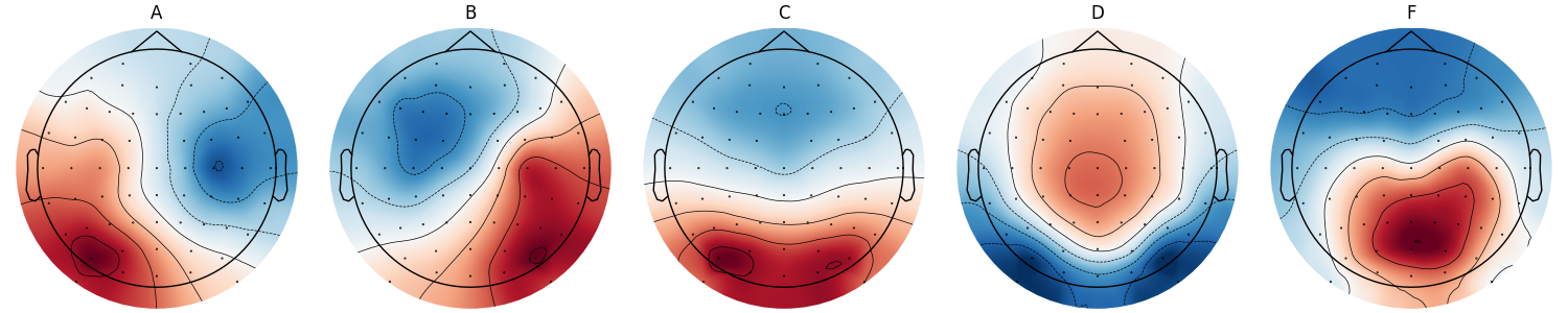
<Figure size 1500x300 with 5 Axes>
The map polarities can be inverted using the
pycrostates.cluster.ModKMeans.invert_polarity().
method. Note that it only affects visualization, it has not effect during
backfitting as polarities are ignored.
ModK.invert_polarity([False, False, True, True, False])
ModK.plot()
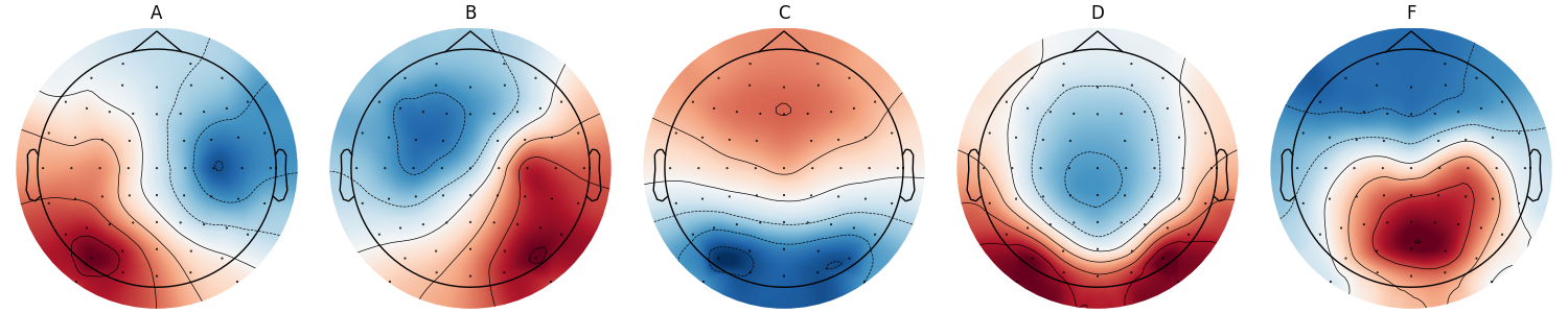
<Figure size 1500x300 with 5 Axes>
Total running time of the script: (0 minutes 11.707 seconds)
Estimated memory usage: 258 MB