Evaluating clustering fits

Since microstate analysis is based on an empirical model, it is impossible to know the ground truth label of each sample. It is therefore necessary to rely on reliable metrics in order to evaluate the relevance of the parameters used in our model, and more particularly the number of cluster centers.

Pycrostates implements several metrics to evaluate the quality of clustering solutions without knowing the ground truth:

• Silhouette score[1]: silhouette_score() (higher the better)

• Calinski-Harabasz score[2]: calinski_harabasz_score() (higher the better)

• Dunn score[3]: dunn_score() (higher the better)

• Davies-Bouldin score[4]: davies_bouldin_score() (lower the better)

Those metrics can directly be applied to a fitted clustering algorithm such as the ModKMeans.

Note

The lemon datasets used in this tutorial is composed of EEGLAB files. To use the MNE reader mne.io.read_raw_eeglab(), the pymatreader optional dependency is required. Use the following installation method appropriate for your environment:

• pip install pymatreader

• conda install -c conda-forge pymatreader

Note that an environment created via the MNE installers includes pymatreader by default.

import matplotlib.pyplot as plt
import numpy as np
from mne import set_log_level
from mne.io import read_raw_eeglab

from pycrostates.cluster import ModKMeans
from pycrostates.datasets import lemon


set_log_level("ERROR")  # reduce verbosity

raw_fname = lemon.data_path(subject_id="010017", condition="EO")
raw = read_raw_eeglab(raw_fname, preload=True)
raw.crop(0, 180)
raw.pick("eeg")
raw.set_eeg_reference("average")

	General
	Filename(s)	sub-010017_EO.fdt
	MNE object type	RawEEGLAB
	Measurement date	Unknown
	Participant	Unknown
	Experimenter	Unknown
	Acquisition
	Duration	00:03:01 (HH:MM:SS)
	Sampling frequency	250.00 Hz
	Time points	45,001
	Channels
	EEG	61
	Head & sensor digitization	64 points
	Filters
	Highpass	0.00 Hz
	Lowpass	125.00 Hz

Intra/Inter cluster distances

Clustering scores often rely on inter-cluster distance and intra-cluster distance. Those concepts can be expanded to define the density of a cluster, or the dispersion of a cluster.

The inter-cluster distance represents the distance between two datapoints belonging to two different clusters.

The intra-cluster distance represents the distance between two datapoints belonging to the same cluster.

Depending on the score used, those distances can be computed in different ways.

Silhouette score

The Silhouette score[1] focuses on 2 metrics: the intra-cluster distance and the inter-cluster distance. It summarizes how well clusters are dense and well separated.

The silhouette score is bounded between -1 (low cluster separation) to 1 (high cluster separation).

Calinski-Harabasz score

The Calinski-Harabasz score[2] is the ratio of the sum of inter-cluster dispersion and of intra-cluster dispersion for all clusters (where the dispersion is defined as the sum of correlations squared). As the silhouette score, it also summarizes how well clusters are dense and well separated. Higher values indicates higher cluster density and better separation.

Dunn score

The Dunn score[3] is defined as a ratio of the smallest inter-cluster distance to the largest intra-cluster distance. Overall, it summarizes how well clusters are farther apart and less dispersed. Higher values indicates a better separation.

Davies-Bouldin score

The Davies-Bouldin score[4] is defined as the average similarity measure of each cluster with its most similar cluster, where similarity is the ratio of intra-cluster distance to inter-cluster distance. Overall, it summarizes how well clusters are farther apart and less dispersed. Lower values indicates a better separation, 0 being the lowest score possible.

Compute scores

In this example, we will use a single subject EEG recording in order to give more explanation about each of this metrics before showing an application case to determine the optimal number of cluster centers n_clusters while fitting a ModKMeans algorithm. For this example, we start by computing each of the score on the clustering results of a ModKMeans fitted for different n_clusters ranging from 2 to 8. To speed-up the fitting while preserving most of the information, only the Global Field Power (GFP) peaks are used.

from pycrostates.metrics import (
    silhouette_score,
    calinski_harabasz_score,
    dunn_score,
    davies_bouldin_score,
)
from pycrostates.preprocessing import extract_gfp_peaks


cluster_numbers = range(2, 9)
scores = {
    "Silhouette": np.zeros(len(cluster_numbers)),
    "Calinski-Harabasaz": np.zeros(len(cluster_numbers)),
    "Dunn": np.zeros(len(cluster_numbers)),
    "Davies-Bouldin": np.zeros(len(cluster_numbers)),
}
gfp_peaks = extract_gfp_peaks(raw)
for k, n_clusters in enumerate(cluster_numbers):
    # fit K-means algorithm with a set number of cluster centers
    ModK = ModKMeans(n_clusters=n_clusters, random_state=42)
    ModK.fit(gfp_peaks, n_jobs=2, verbose="WARNING")

    # compute scores
    scores["Silhouette"][k] = silhouette_score(ModK)
    scores["Calinski-Harabasaz"][k] = calinski_harabasz_score(ModK)
    scores["Dunn"][k] = dunn_score(ModK)
    scores["Davies-Bouldin"][k] = davies_bouldin_score(ModK)

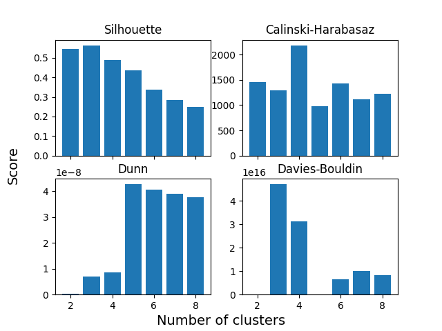
Plot individual scores

We can plot the different scores with matplotlib.pyplot.bar().

f, ax = plt.subplots(2, 2, sharex=True)
for k, (score, values) in enumerate(scores.items()):
    ax[k // 2, k % 2].bar(x=cluster_numbers, height=values)
    ax[k // 2, k % 2].set_title(score)
plt.text(
    0.03,
    0.5,
    "Score",
    horizontalalignment="center",
    verticalalignment="center",
    rotation=90,
    fontdict=dict(size=14),
    transform=f.transFigure,
)
plt.text(
    0.5,
    0.03,
    "Number of clusters",
    horizontalalignment="center",
    verticalalignment="center",
    fontdict=dict(size=14),
    transform=f.transFigure,
)
plt.show()

Compare scores

We can compare the different scores on a barplot using matplotlib.pyplot.bar(). However, each score spans a different scale, often several order of magnitude different from the others. First, we will normalize each score to unit norm. Except for Davies-Bouldin score, the general rule is the higher the better. Thus, the Davies-Bouldin scores will be inverted.

# invert davies-bouldin scores
scores["Davies-Bouldin"] = 1 / (1 + scores["Davies-Bouldin"])

# normalize scores using sklearn
from sklearn.preprocessing import normalize

scores = {
    score: normalize(value[:, np.newaxis], axis=0).ravel()
    for score, value in scores.items()
}

# set width of a bar and define colors
barWidth = 0.2
colors = ["#4878D0", "#EE854A", "#6ACC64", "#D65F5F"]

# create figure
plt.figure(figsize=(10, 8))
# create the position of the bars on the X-axis
x = [
    [elt + k * barWidth for elt in np.arange(len(cluster_numbers))]
    for k in range(len(scores))
]
# create plots
for k, (score, values) in enumerate(scores.items()):
    plt.bar(
        x=x[k],
        height=values,
        width=barWidth,
        edgecolor="grey",
        color=colors[k],
        label=score,
    )
# add labels and legend
plt.xlabel("Number of clusters")
plt.ylabel("Score normalize to unit norm")
plt.xticks(
    [pos + 1.5 * barWidth for pos in range(len(cluster_numbers))],
    [str(k) for k in cluster_numbers],
)
plt.legend()
plt.show()

Conclusion

There is no global consensus on which n_cluster value to choose. The Silhoutette score seems to be in favor of n_clusters=3, Calinski-Harabasz score n_clusters=4, Dunn score n_clusters=5 and Davies-Bouldin score n_clusters=2 or 5. Each of these scores provides similar but different information about the quality of the clustering.

Note that for microstate analysis the choice of the number of cluster centers is also a trade off between the quality of the clustering, interpretations that can be made of it, and the variance expressed by the current clustering. There isn’t an ideal solution and it is up to the person who conducts the analysis to evaluate the most judicious choice, by exploring for example several clustering solutions.

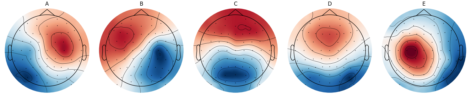
Microstates fitted for n=5

In this case, n_clusters=5 seems like a reasonable choice. This number of clusters yields the following maps:

ModK = ModKMeans(n_clusters=5, random_state=42)
ModK.fit(gfp_peaks, n_jobs=2, verbose="WARNING")

ModK.reorder_clusters(order=[4, 1, 3, 0, 2])
ModK.rename_clusters(new_names=["A", "B", "C", "D", "E"])
ModK.plot()

<Figure size 1500x300 with 5 Axes>

References

[1] (1,2)

Peter J. Rousseeuw. Silhouettes: a graphical aid to the interpretation and validation of cluster analysis. Journal of Computational and Applied Mathematics, 20:53–65, 1987. doi:10.1016/0377-0427(87)90125-7.

[2] (1,2)

T. Caliński and J. Harabasz. A dendrite method for cluster analysis. Communications in Statistics, 3(1):1–27, 1974. doi:10.1080/03610927408827101.

[3] (1,2)

J. C. Dunn†. Well-separated clusters and optimal fuzzy partitions. Journal of Cybernetics, 4(1):95–104, 1974. doi:10.1080/01969727408546059.

[4] (1,2)

David L. Davies and Donald W. Bouldin. A cluster separation measure. IEEE Transactions on Pattern Analysis and Machine Intelligence, PAMI-1(2):224–227, 1979. doi:10.1109/TPAMI.1979.4766909.

Estimated memory usage: 689 MB