pycrostates.segmentation.RawSegmentation#

class pycrostates.segmentation.RawSegmentation(*args, **kwargs)[source]#

Contains the segmentation of a Raw instance.

Parameters:

labelsarray of shape (n_samples,): Microstates labels attributed to each sample, i.e. the segmentation.
rawRaw: Raw instance used for prediction.
cluster_centersarray (n_clusters, n_channels): Clusters, i.e. the microstates maps used to compute the segmentation.
cluster_nameslist | None: Name of the clusters.
predict_parametersdict | None: The prediction parameters.

Attributes:

cluster_centers_: Cluster centers (i.e topographies) used to compute the segmentation.
cluster_names: Name of the cluster centers.
labels: Microstate label attributed to each sample (the segmentation).
predict_parameters: Parameters used to predict the current segmentation.
raw: Raw instance from which the segmentation was computed.

Methods

`compute_expected_transition_matrix`([stat, ...])	Compute the expected transition matrix.
`compute_parameters`([norm_gfp, return_dist])	Compute microstate parameters.
`compute_transition_matrix`([stat, ...])	Compute the observed transition matrix.
`entropy`([ignore_repetitions, log_base])	Compute the Shannon entropy of the segmentation.
`plot`([tmin, tmax, cmap, axes, cbar_axes, ...])	Plot the segmentation.
`plot_cluster_centers`([axes, block, show])	Plot cluster centers as topographic maps.

compute_expected_transition_matrix(stat='probability', ignore_repetitions=True)#

Compute the expected transition matrix.

Compute the theoretical transition matrix as if time course was ignored, but microstate proportions kept (i.e. shuffled segmentation). This matrix can be used to quantify/correct the effect of microstate time coverage on the observed transition matrix obtained with the method compute_expected_transition_matrix. Transition “from” and “to” unlabeled segments -1 are ignored.

Parameters:

statstr

Aggregate statistic to compute transitions. Can be:

probability or proportion: normalize count such as the probabilities along the first axis is always equal to 1.
percent: normalize count such as the probabilities along the first axis is always equal to 100.

ignore_repetitionsbool

If True, ignores state repetitions. For example, the input sequence AAABBCCD will be transformed into ABCD before any calculation. This is equivalent to setting the duration of all states to 1 sample.

Returns:

Tarray of shape (n_cluster, n_cluster): Array of transition probability values from one label to another. First axis indicates state "from". Second axis indicates state "to".

compute_parameters(norm_gfp=True, return_dist=False)#

Compute microstate parameters.

Warning

When working with Epochs, this method will put together segments of all epochs. This could lead to wrong interpretation especially on state durations. To avoid this behaviour, make sure to set the reject_edges parameter to True when creating the segmentation.

Parameters:

norm_gfpbool: If True, the global field power (GFP) is normalized.
return_distbool: If True, return the parameters distributions.

Returns:

dictdict

Dictionaries containing microstate parameters as key/value pairs. Keys are named as follow: '{microstate name}_{parameter name}'.

Available parameters are listed below:

mean_corr: Mean correlation value for each time point assigned to a given state.
gev: Global explained variance expressed by a given state. It is the sum of global explained variance values of each time point assigned to a given state.
timecov: Time coverage, the proportion of time during which a given state is active. This metric is expressed as a ratio.
meandurs: Mean durations of segments assigned to a given state. This metric is expressed in seconds (s).
occurrences: Occurrences per second, the mean number of segment assigned to a given state per second. This metrics is expressed in segment per second.
dist_corr (req. return_dist=True): Distribution of correlations values of each time point assigned to a given state.
dist_gev (req. return_dist=True): Distribution of global explained variances values of each time point assigned to a given state.
dist_durs (req. return_dist=True): Distribution of durations of each segments assigned to a given state. Each value is expressed in seconds (s).

compute_transition_matrix(stat='probability', ignore_repetitions=True)#

Compute the observed transition matrix.

Count the number of transitions from one state to another and aggregate the result as statistic. Transition “from” and “to” unlabeled segments -1 are ignored.

Parameters:

%(stat_transition)s
%(ignore_repetitions)s

Returns:

%(transition_matrix)s

Notes

Warning

When working with Epochs, this method will take into account transitions that occur between epochs. This could lead to wrong interpretation when working with discontinuous data. To avoid this behaviour, make sure to set the reject_edges parameter to True when predicting the segmentation.

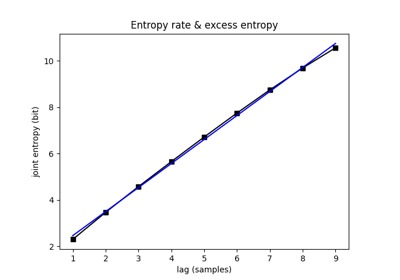
entropy(ignore_repetitions=False, log_base=2)#

Compute the Shannon entropy of the segmentation.

Compute the Shannon entropy[1] of the microstate symbolic sequence.

Parameters:

ignore_repetitionsbool: If True, ignores state repetitions. For example, the input sequence AAABBCCD will be transformed into ABCD before any calculation. This is equivalent to setting the duration of all states to 1 sample.
log_basefloat | str: The log base to use. If string: * bits: log_base = 2 * natural: log_base = np.e * dits: log_base = 10 Default to bits.

Returns:

hfloat: The Shannon entropy.

References

plot(tmin=None, tmax=None, cmap=None, axes=None, cbar_axes=None, *, block=False, show=None, verbose=None)[source]#

Plot the segmentation.

Parameters:

tminfloat: Start time of the raw data to use in seconds (must be >= 0).
tmaxfloat | None: End time of the raw data to use in seconds (cannot exceed data duration). If None (default), the current end of the data is used.
cmapstr | colormap | None: The colormap to use. If None, viridis is used.
axesAxes | None: Either None to create a new figure or axes on which the segmentation is plotted.
cbar_axesAxes | None: Axes on which to draw the colorbar, otherwise the colormap takes space from the main axes.
blockbool: Whether to halt program execution until the figure is closed.
showbool | None: If True, the figure is shown. If None, the figure is shown if the matplotlib backend is interactive.
verboseint | str | bool | None: Sets the verbosity level. The verbosity increases gradually between "CRITICAL", "ERROR", "WARNING", "INFO" and "DEBUG". If None is provided, the verbosity is set to "WARNING". If a bool is provided, the verbosity is set to "WARNING" for False and to "INFO" for True.

Returns:

figFigure: Matplotlib figure containing the segmentation.

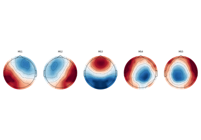
plot_cluster_centers(axes=None, *, block=False, show=None)#

Plot cluster centers as topographic maps.

Parameters:

axesAxes | None: Either None to create a new figure or axes (or an array of axes) on which the topographic map should be plotted. If the number of microstates maps to plot is ≥ 1, an array of axes of size n_clusters should be provided.
blockbool: Whether to halt program execution until the figure is closed.
showbool | None: If True, the figure is shown. If None, the figure is shown if the matplotlib backend is interactive.

Returns:

figFigure: Matplotlib figure containing the topographic plots.

property cluster_centers_#

Cluster centers (i.e topographies) used to compute the segmentation.

Type:: array

property cluster_names#

Name of the cluster centers.

Type:: list

property labels#

Microstate label attributed to each sample (the segmentation).

Type:: array

property predict_parameters#

Parameters used to predict the current segmentation.

Type:: dict

property raw#: Raw instance from which the segmentation was computed.

Examples using `pycrostates.segmentation.RawSegmentation`#

Group-level analysis from individual clusters

Group level analysis from individual GFP peaks

Microstate Segmentation

Entropy and related measures

pycrostates.segmentation.RawSegmentation#

Examples using pycrostates.segmentation.RawSegmentation#

Examples using `pycrostates.segmentation.RawSegmentation`#