Subject level analysis with resampling

This tutorial introduces how to use pycrostates.preprocessing.resample to compute individual microstate topographies and study the stability of the clustering results.

Note

The lemon datasets used in this tutorial is composed of EEGLAB files. To use the MNE reader mne.io.read_raw_eeglab(), the pymatreader optional dependency is required. Use the following installation method appropriate for your environment:

• pip install pymatreader

• conda install -c conda-forge pymatreader

Note that an environment created via the MNE installers includes pymatreader by default.

import numpy as np
from matplotlib import pyplot as plt
from mne.io import read_raw_eeglab

from pycrostates.cluster import ModKMeans
from pycrostates.datasets import lemon


raw_fname = lemon.data_path(subject_id="010017", condition="EC")
raw = read_raw_eeglab(raw_fname, preload=True)
raw.crop(0, 60)
raw.pick("eeg")
raw.set_eeg_reference("average")

/home/docs/checkouts/readthedocs.org/user_builds/pycrostates/checkouts/main/tutorials/cluster/10_subject_level_with_resampling.py:35: RuntimeWarning: Limited 1 annotation(s) that were expanding outside the data range.
  raw = read_raw_eeglab(raw_fname, preload=True)
/home/docs/checkouts/readthedocs.org/user_builds/pycrostates/checkouts/main/tutorials/cluster/10_subject_level_with_resampling.py:35: RuntimeWarning: The data contains 'boundary' events, indicating data discontinuities. Be cautious of filtering and epoching around these events.
  raw = read_raw_eeglab(raw_fname, preload=True)

	General
	Filename(s)	sub-010017_EC.fdt
	MNE object type	RawEEGLAB
	Measurement date	Unknown
	Participant	Unknown
	Experimenter	Unknown
	Acquisition
	Duration	00:01:01 (HH:MM:SS)
	Sampling frequency	250.00 Hz
	Time points	15,001
	Channels
	EEG	61
	Head & sensor digitization	64 points
	Filters
	Highpass	0.00 Hz
	Lowpass	125.00 Hz

Resampling is a technique which consist of selecting a subset from a dataset several times. This method can be useful to study the stability and reliability of clustering results. In this example, we will split our data in n_resamples resamples each containing n_samples randomly selected from the original recording.

Note

This method can also be used on GFP peaks only!

gfp_peaks = pycrostates.preprocessing.extract_gfp_peaks(raw)
resamples = resample(
    gfp_peaks, n_resamples=3, n_samples=1000, random_state=42
)

from pycrostates.preprocessing import resample

resamples = resample(raw, n_resamples=3, n_samples=1000, random_state=42)

We can compute the cluster centers on each of the resample and plot the topographic maps fitted on a unique figure with the axes argument.

f, ax = plt.subplots(nrows=len(resamples), ncols=5)

resample_results = []
for k, resamp in enumerate(resamples):
    # fit Modified K-means
    ModK = ModKMeans(n_clusters=5, random_state=42)
    ModK.fit(resamp, n_jobs=2, verbose="WARNING")
    resample_results.append(ModK.cluster_centers_)
    # plot the cluster centers
    fig = ModK.plot(axes=ax[k, :])
    plt.text(
        0.5,
        1.4,
        f"GEV: {ModK.GEV_:.2f}",
        horizontalalignment="center",
        verticalalignment="center",
        transform=ax[k, 2].transAxes,
        fontdict=dict(size=14),
    )

plt.subplots_adjust(top=0.9, hspace=0.5)
plt.show()

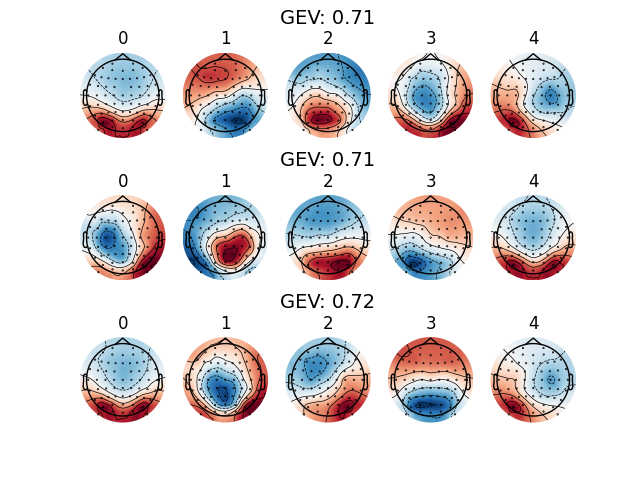
Each resampling clustering solution explains about 70% of its Global Explained Variance (GEV). We can distinguish similar topographies between fits, although with large variation, different signs and in a different order. The sparsity of results reveals how data sampling may influence the results of microstates analysis. Sampling issues are inherent to EEG recording: recording are conducted at a specific time a specific day, in specific condition and have a finite duration.

To improve the stability of the clustering, it is possible to compute a second clustering solution on the concatenated cluster centers fitted on the resample datasets.

from pycrostates.io import ChData

all_resampling_results = np.vstack(resample_results).T
all_resampling_results = ChData(all_resampling_results, raw.info)

ModK = ModKMeans(n_clusters=5, random_state=42)
ModK.fit(all_resampling_results, n_jobs=2, verbose="WARNING")
ModK.plot()

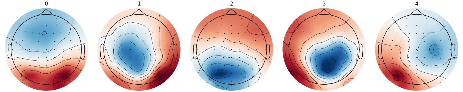
<Figure size 1500x300 with 5 Axes>

Note

This method can also be applied for group level analysis by mixing individual resampling results together.

Estimated memory usage: 202 MB